%matplotlib inline

import stistools
from astropy.io import fits
import matplotlib.pyplot as plt
import numpy as np
import glob
import matplotlib
matplotlib.rcParams['image.origin'] = 'lower'
matplotlib.rcParams['image.aspect'] = 'auto'
matplotlib.rcParams['image.cmap'] = 'plasma'
matplotlib.rcParams['image.interpolation'] = 'none'
matplotlib.rcParams['figure.figsize'] = [15, 5]
STIS CCD Defringing Examples
The Stistools defringing tools
(normspflat,prepspec,mkfringeflat, and defringe) are
needed to correct the fringing patterns that are present in the reddest
STIS observing modes (>7000 ), namely G750M and
G750L. The Defringing Guide provides a step-by-step tutorial on how to
use these tools to perform this correction. The following serves to show
several practical examples of it’s use on STIS data.
), namely G750M and
G750L. The Defringing Guide provides a step-by-step tutorial on how to
use these tools to perform this correction. The following serves to show
several practical examples of it’s use on STIS data.
G750L Observation of HZ43
# Set up the data paths

sci_file = 'o49x18010'
flat_file = 'o49x18020'

# Normalize the contemoraneous flat field image
stistools.defringe.normspflat(f"{flat_file}_raw.fits",
                              f"{flat_file}_nsp.fits", do_cal=True,
                              wavecal=f"{sci_file}_wav.fits")
File written: /Users/stisuser/data/path/o49x18020_crj.fits
# make the fringe flat, using the crj file for the science because this is G750L
stistools.defringe.mkfringeflat(f"{sci_file}_crj.fits", f"{flat_file}_nsp.fits",
                               f"{flat_file}_frr.fits")
mkfringeflat.py version 0.1
 - matching fringes in a flatfield to those in science data
 Extraction center: row 511
   Extraction size: 11.0 pixels  [Aperture: 52X2]
Range to be normalized: [506:517,4:1020]

Determining best shift for fringe flat

shift = -0.5, rms = 0.02521565587012733
shift = -0.4, rms = 0.02374587534351394
shift = -0.3, rms = 0.022735165926832522
shift = -0.19999999999999996, rms = 0.022235801562053452
shift = -0.09999999999999998, rms = 0.0223095350312966
shift = 0.0, rms = 0.022870072599462554
shift = 0.10000000000000009, rms = 0.023099186545412927
shift = 0.20000000000000007, rms = 0.0238499817578987
shift = 0.30000000000000004, rms = 0.025041375073110203
shift = 0.4, rms = 0.026649802114317847
shift = 0.5, rms = 0.02860146728021774

 Best shift : -0.1963593679893798 pixels
 Shifted flat : o49x18020_nsp_sh.fits
                (Can be used as input flat for next iteration)

Determining best scaling of amplitude of fringes in flat

Fringes scaled  0.8: RMS = 0.022225777873537036
Fringes scaled  0.8400000000000001: RMS = 0.021245650237594484
Fringes scaled  0.88: RMS = 0.02073729355208867
Fringes scaled  0.92: RMS = 0.02073643145196044
Fringes scaled  0.9600000000000001: RMS = 0.021244380189719227
Fringes scaled  1.0: RMS = 0.022227696178223795
Fringes scaled  1.04: RMS = 0.023664059746596907
Fringes scaled  1.08: RMS = 0.025413279490181823
Fringes scaled  1.12: RMS = 0.02744748231768354
Fringes scaled  1.1600000000000001: RMS = 0.029710009708226032
Fringes scaled  1.2000000000000002: RMS = 0.03215458872298658

 Best scale : 0.9182259885801685
Output flat : o49x18020_frr.fits
  (to be used as input to task 'defringe.py')
# Defringe the science spectrum
stistools.defringe.defringe(f"{sci_file}_crj.fits", f"{flat_file}_frr.fits", overwrite=True)
Fringe flat data were read from the primary HDU
Imset 1 done
Defringed science saved to o49x18010_drj.fits
'o49x18010_drj.fits'
# Now, extract the spectra from both the fringed (crj) and defringed (drj) data
defringed = glob.glob(f"{sci_file}*drj.fits")
fringed = glob.glob(f"{sci_file}*crj.fits")
files = [defringed[0], fringed[0]]

outnames = [f'{defringed[0].split("/")[-1].split("_")[0]}_dx1d.fits', f'{fringed[0].split("/")[-1].split("_")[0]}_x1d.fits']

for i in range(len(outnames)):
    stistools.x1d.x1d(files[i], output=outnames[i])
dx1d = fits.open(outnames[0])
x1d = fits.open(outnames[1])
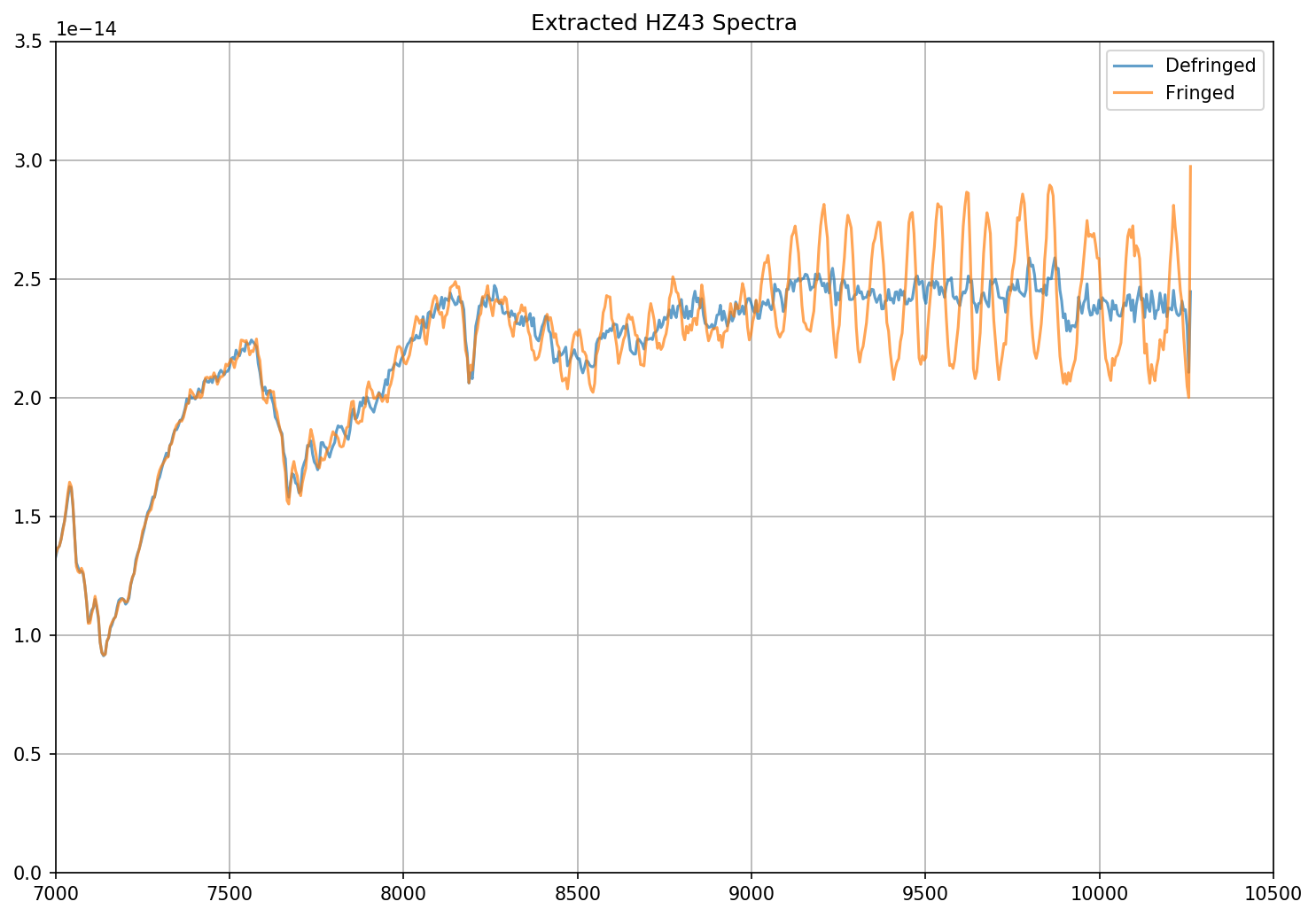
# Plot both the fringed and the defringed 1D extracted spectra together
fig = plt.figure(figsize=(10,7),dpi=150)
plt.plot(dx1d[1].data['WAVELENGTH'][0], dx1d[1].data['FLUX'][0],'-', label='Defringed', alpha=0.7)
plt.plot(x1d[1].data['WAVELENGTH'][0], x1d[1].data['FLUX'][0],'-', label='Fringed', alpha=0.7)
plt.xlim(7000,10500)
plt.ylim(0, 3.5e-14)
plt.title("Extracted HZ43 Spectra")
plt.grid()
plt.legend()
plt.tight_layout()
G750M Observation of AGK+81D266
#setup data paths

sci_file = "oe36m10g0"
flat_file = "oe36m10j0"

# Normalize the contemporaneous flat field image
stistools.defringe.normspflat(f"{flat_file}_raw.fits",
                              f"{flat_file}_nsp.fits", do_cal=True,
                              wavecal=f"{sci_file}_wav.fits")
File written: /Users/stisuser/data/path/oe36m10j0_sx2.fits
/Users/stisuser/install/path/normspflat.py:216: RuntimeWarning: divide by zero encountered in true_divide
  row_fit = fit_data/spl(xrange)
/Users/stisuser/install/path/normspflat.py:216: RuntimeWarning: invalid value encountered in true_divide
  row_fit = fit_data/spl(xrange)
# make the fringe flat, using the sx2 file for the science because this is G750M
stistools.defringe.mkfringeflat(f"{sci_file}_sx2.fits", f"{flat_file}_nsp.fits",
                                f"{flat_file}_frr.fits", beg_shift=-1.0, end_shift=0.5, shift_step=0.1,
                                beg_scale=0.8, end_scale=1.5, scale_step=0.04)
mkfringeflat.py version 0.1
 - matching fringes in a flatfield to those in science data
 Extraction center: row 602
   Extraction size: 11.0 pixels  [Aperture: 52X2]
Range to be normalized: [597:608,83:1106]

Determining best shift for fringe flat

shift = -1.0, rms = 0.06751209969416246
shift = -0.9, rms = 0.06750664734039523
shift = -0.8, rms = 0.06750325556538965
shift = -0.7, rms = 0.06750192457752245
shift = -0.6, rms = 0.06750265937240976
shift = -0.5, rms = 0.06750545682621624
shift = -0.3999999999999999, rms = 0.06750588470469428
shift = -0.29999999999999993, rms = 0.06751357970780972
shift = -0.19999999999999996, rms = 0.06752336035281563
shift = -0.09999999999999998, rms = 0.06753522897336409
shift = 0.0, rms = 0.06754918994601025
shift = 0.10000000000000009, rms = 0.06754304260847464
shift = 0.20000000000000018, rms = 0.0675389748466461
shift = 0.30000000000000004, rms = 0.06753698522431144
shift = 0.40000000000000013, rms = 0.06753708053436966
shift = 0.5, rms = 0.06753925625176614

 Best shift : -0.6999982359381194 pixels
 Shifted flat : oe36m10j0_nsp_sh.fits
                (Can be used as input flat for next iteration)

Determining best scaling of amplitude of fringes in flat

Fringes scaled  0.8: RMS = 0.06762238400706264
Fringes scaled  0.8400000000000001: RMS = 0.06759376871355414
Fringes scaled  0.88: RMS = 0.06756741543477168
Fringes scaled  0.92: RMS = 0.0675433153759303
Fringes scaled  0.9600000000000001: RMS = 0.06752149090813866
Fringes scaled  1.0: RMS = 0.06750192634866954
Fringes scaled  1.04: RMS = 0.067484628741123
Fringes scaled  1.08: RMS = 0.06746960905640136
Fringes scaled  1.12: RMS = 0.06745685643406156
Fringes scaled  1.1600000000000001: RMS = 0.06744637965688902
Fringes scaled  1.2000000000000002: RMS = 0.06743817834085863
Fringes scaled  1.24: RMS = 0.06743225706483276
Fringes scaled  1.28: RMS = 0.06742860539788004
Fringes scaled  1.32: RMS = 0.06742723706558065
Fringes scaled  1.36: RMS = 0.06742814340085584
Fringes scaled  1.4: RMS = 0.06743132876996823
Fringes scaled  1.44: RMS = 0.06743679508124968
Fringes scaled  1.48: RMS = 0.06744453855109715
Fringes scaled  1.52: RMS = 0.06745456004413491

 Best scale : 1.3200005501263359
Output flat : oe36m10j0_frr.fits
  (to be used as input to task 'defringe.py')
# defringe the science spectrum
stistools.defringe.defringe(f"{sci_file}_sx2.fits", f"{flat_file}_frr.fits", overwrite=True)
Fringe flat data were read from the primary HDU
19 pixels in the fringe flat were less than or equal to 0
Imset 1 done
Defringed science saved to oe36m10g0_s2d.fits
/Users/stisuser/install/path/defringe.py:95: RuntimeWarning: invalid value encountered in less_equal
  fringe_mask = (fringe_data <= 0.)
'oe36m10g0_s2d.fits'
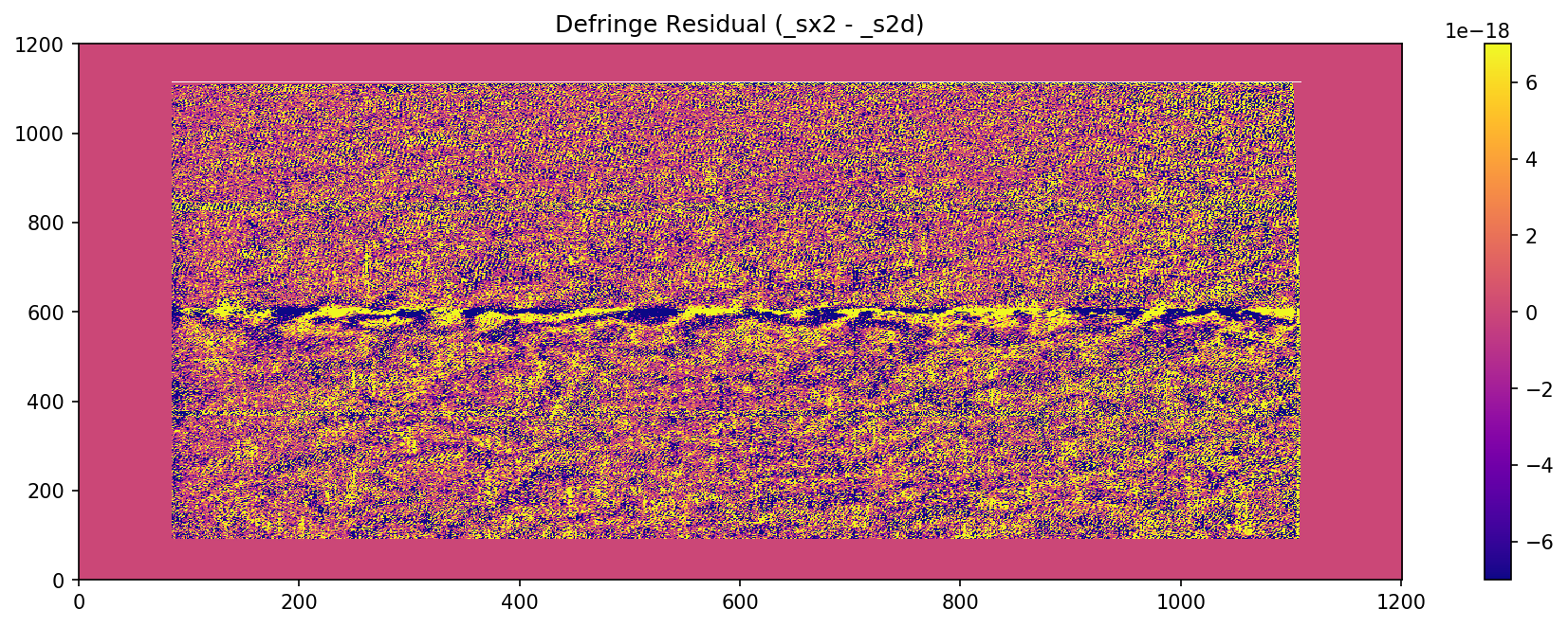
# Plot the fringe pattern removed from the sx2 file

scale = 7*10**-18
resid = fits.getdata(f"{sci_file}_sx2.fits")-fits.getdata(f"{sci_file}_s2d.fits")

fig = plt.figure(dpi=150)
plt.imshow(resid,vmin=-scale, vmax=scale)
plt.title("Defringe Residual (_sx2 - _s2d)")

cbar = plt.colorbar()